Difference between revisions of "Image Synthesis"
(→Project 1) |
(→Project 14) |
||
| (14 intermediate revisions by the same user not shown) | |||
| Line 1: | Line 1: | ||
I took this class with [http://psgraphics.blogspot.com/ Dr. Pete Shirley] in 2006. He was a very animated professor and loved talking about light and how it behaved. At one point I remember him mid sentence running into the kitchen connected to our classroom and coming back with a glass container he held up looking at it from different angles to talk about refraction. | I took this class with [http://psgraphics.blogspot.com/ Dr. Pete Shirley] in 2006. He was a very animated professor and loved talking about light and how it behaved. At one point I remember him mid sentence running into the kitchen connected to our classroom and coming back with a glass container he held up looking at it from different angles to talk about refraction. | ||
| − | All of the assignments were completed via blog postings. I decided to write my renderer in java for kicks, while most people chose to use C++. Looking back I slightly regret my decision since I had no experience writing "fast" java code and my renders took noticeably longer than my classmates. | + | All of the assignments were completed via blog postings. I decided to write my renderer in java for kicks, while most people chose to use C++. Looking back I slightly regret my decision since I had no experience writing "fast" java code and my renders took noticeably longer than my classmates. Still it was one of the funnest college courses I had. |
== Project 1 == | == Project 1 == | ||
| Line 9: | Line 9: | ||
[[File:im_synth_p1_s1.png|thumb|center|1 Sample]] | [[File:im_synth_p1_s1.png|thumb|center|1 Sample]] | ||
| − | [[File:im_synth_p1_s16.png|thumb|16 Samples]] | + | [[File:im_synth_p1_s16.png|thumb|center|16 Samples]] |
| − | [[File:im_synth_p1_s256.png|thumb|256 Samples]] | + | [[File:im_synth_p1_s256.png|thumb|center|256 Samples]] |
| − | [[File:im_synth_p1_s1024.png|thumb|1024 Samples]] | + | [[File:im_synth_p1_s1024.png|thumb|center|1024 Samples]] |
== Project 2 == | == Project 2 == | ||
| Line 19: | Line 19: | ||
This second project is similar to the first. I sampled XYZ estimates using the tristimulus curves and converted the samples on the graphics card to RGB using the Adobe RGB table conversion standard matrix. It took my poor little laptop almost two minutes to render 1024 time steps at 720x480. | This second project is similar to the first. I sampled XYZ estimates using the tristimulus curves and converted the samples on the graphics card to RGB using the Adobe RGB table conversion standard matrix. It took my poor little laptop almost two minutes to render 1024 time steps at 720x480. | ||
| − | [[File: | + | [[File:im_synth_p2_s16.png|thumb|center|16 Samples]] |
| − | [[File: | + | [[File:im_synth_p2_s256.png|thumb|center|256 Samples]] |
| − | [[File: | + | [[File:im_synth_p2_s1024.png|thumb|center|1024 Samples]] |
| − | [[File: | + | == Project 3 == |
| + | |||
| + | These are samples from a simulated sensor. The grid is on the xy-plane and a sphere emitting light from it's surface at random vectors hits the sensor grid and accumulates XYZ factors, which are converted to RGB on the graphics card and displayed to the screen. Below are images of this program taken at different number of photon emissions. | ||
| + | |||
| + | [[File:im_synth_p3_s1000.png|frame|center|1,000 Emissions]] | ||
| + | |||
| + | [[File:im_synth_p3_s1000000.png|frame|center|1,000,000 Emissions]] | ||
| + | |||
| + | [[File:im_synth_p3_s100000000.png|frame|center|100,000,000 Emissions]] | ||
| + | |||
| + | == Project 4 and 5 == | ||
| + | |||
| + | In the previous project, a single sphere-shaped light emitter was placed onto the sensor grid. In the example, the light source has been moved back and a pinhole has been added between the sensor grid and all other objects in the scene. This pinhole only allows vectors of photons pass through it if it they travel inside the pinhole to reach the grid. Other photons are thrown out. This pinhole-camera scheme provides a much better detailed picture than the previous implementation as it simulates a perspective frustrum just like the eye or a real camera. A red diffuse sphere bounces light from the light source to the pinhole also. | ||
| + | |||
| + | Included in this project was an importance sampling implementation. This fired photons at the diffuse sphere and directly at the pinhole. The amount of photons fired to each object was a ratio of their solid angle and the total number of photons previously fired in all directions. Because only photons sent to the pinhole and the object were fired, the scene was rendered using much fewer photons. Although more overhead was required to calculate the importance sampling, it greatly reduced the calculation time for every photon collision (having much fewer photons in the scene). | ||
| + | |||
| + | Both of these projects were added to the previous code base at the same time. Importance sampling was required to provide an more interactive debugging of the pinhole code. Final images look better than the previous project, and took much less time to synthesize. | ||
| + | |||
| + | [[File:im_synth_p4_is.png|frame|center|313,290,000 emissions (876,964 passed through the pinhole)]] | ||
| + | |||
| + | == Project 6 and 15 == | ||
| + | |||
| + | In Project 4 & 5, the imager was modified to handle importance sampling and a pinhole camera. The importance sampling provided much faster rendering times by sending photons only at known objects in the scene, and weighting them based on their angle. The photons were generated at the sensor grid and sent through the scene until they hit a light source (or bounced too much). This seemed to provide a good sampling of the scene, but required a major rewrite of the code. | ||
| + | |||
| + | This new version of the software adds a lens to the scene as well as motion blur. To handle motion blur, the red diffuse sphere was moved from (0, 1, 3) to (1, 2, 4) over the course of the rendering. This created an easy but interesting blur effect as if the object was exposed over many sensor units while the apperture was open. | ||
| + | |||
| + | The lense was a simple biconvex lense attached to the pinhole. Upon contact with the lense, the vector was skewed based on it's angle of incidence and the refractive index of the lense (1.4 for this lense). As the photon left this lense, it would be skewed again. Snell's law was used to calculate the angles of refraction for each photon. | ||
| + | |||
| + | [[File:im_synth_p6_is.png|frame|center|Rendered using 18,000,000,000 photons -- 200,000 per sensor grid (4 hours, 11 seconds rendering time)]] | ||
| + | |||
| + | == Project 7 and 8 == | ||
| + | |||
| + | In Project 7, we were to use our renderer to model the Cornell box. This box was compared against a physical model to compare accuracy in the rendering software. This scene's walls and light are modeled using the geometry data and color data from the Cornell box at http://www.graphics.cornell.edu/online/box/data.html. | ||
| + | |||
| + | In addition to the light source and the walls, Project 8 added fresnel effects to the renderer. Instead of the two blocks found in the original Cornell box, two diffuse spheres have been placed in the far corners of the room. A large transparent sphere is placed in the center of the room, which shows the light refracting through it. | ||
| + | |||
| + | The scene's light seems rather blurry because it was moved down slightly to not create artifacts with the ceiling, which is one giant polygon. | ||
| + | |||
| + | [[File:im_synth_p7_cb.png|frame|center|rendered at 400x400 and tone mapped. It took 4 hours to render, which is rather sad]] | ||
| + | |||
| + | == Project 9 == | ||
| + | |||
| + | In Project 9, we were to add the Beere-Lambert Law to our renderer. The Beere-Lambert Law models the amount of light absorbed while traveling through a medium. Because different wavelengths are absorbed based on the distance they must travel through the medium, different colors can be absorbed causing different wavelengths to be more pronounced. Certain types of glass often absorb high and low wavelengths leaving a greenish tint at certain angles. Usually this effect can be seen when the light is going through the greatest distance of the glass. To compute the absorbtion at certain frequencies, euler's number e was taken to the exponent of the distance times a large negative constant (which changes based on the scene metrics). | ||
| + | |||
| + | In the picture below, five spheres are modeled. The back left sphere is a reflective sphere, while the back right is a diffuse sphere. Theses spheres are only to provide background to the scene. The spheres in front are used for comparison. The left sphere is a diffuse/reflective sphere with a purplish hue. The middle sphere is a translucent sphere that implements the Beere-Lambert Law based on the distance of the medium. This gives the sphere the slightly greenish tint. The sphere on the right is also a translucent sphere, but does not implement the Beere-Lambert Law. This was to show the difference in hues generated by this principle. | ||
| + | |||
| + | [[File:im_synth_p9_beere.png|frame|center|This figure shows several spheres. The front-middle sphere uses the Beere-Lambert Law to absorb certain frequencies of light. The front-right sphere has the same parameters as this sphere, except it does not implement the Beere-Lambert Law. This image took 5 hours and 24 minutes to render]] | ||
| + | |||
| + | |||
| + | == Project 10 == | ||
| + | |||
| + | In Project 10, we were to implement participating media. Participating media involves computing physical bounces of light in media such as fog, dust, smoke, etc. where the light bounces around inside the volume instead of just diffusing, reflecting, or refracting. | ||
| + | |||
| + | To implement this, I used the standard marching technique through an axis-aligned bounding box. A ray was sampled multiple times across its vector using small steps. When these steps were inside the bounding volume, they probabilisitcally hit some of the media. | ||
| + | |||
| + | [[File:im_synth_p10_pm.png|frame|center|Participating media is used to simulate a gaseous volume under the cube. Right now my code is very ineffecient and took six hours to get these results. Earlier images not requiring participating media required far less time to converge]] | ||
| + | |||
| + | == Project 11 == | ||
| + | |||
| + | In Project 11, subsurface scattering is added to the renderer. This implies that light hitting the surface of the material enters and bounces around inside the medium before exiting. Many materials such as grapes, skin and marble exhibit this quality. Subsurface scattering in this implementation used ray marching, where the ray enters the medium and bounces around until exiting. Because the ray actually bounced around inside the object instead of just off the surface, the rendering was far more computationally expensive than rendering this scene without SSC. | ||
| + | |||
| + | [[File:im_synth_p11_scatter.png|frame|center|Two spheres are placed side by side with a large rectangular light source placed overhead. The sphere on the left uses subsurface scattering while the sphere on the right uses just Lambertian reflections. Light shining from above simply bounces of the top of the Lambertian sphere, leaving the bottom dark and unilluminated. The SSC sphere, however, has light shining through the medium and appearing at the bottom of the sphere as many materials would]] | ||
| + | |||
| + | == Project 12 == | ||
| + | |||
| + | In Project 12, the Heyney-Greenstein Phase Function was implemented in the renderer. The Heyney-Greenstein Phase Function (HGPF) is an imperical formula to simulate diffuse and specular reflection for a variety of materials using only two parameters. This function uses these these two parameters stored in each object and takes the incidence angle as input. This provides a much greater flexibility for different materials than using the simpler Lambertian reflection. | ||
| + | |||
| + | Finding little data as to proper values, I rendered an image using a wide range of values. From the image generated, it appears a high g-value seems important to produce a good image. This component supposedly relates directly to the angle where most of the light is leaving. It seems natural that a g-value closer to 1 will produce better pictures where light bounces off at a 90-degree angle, while a 0 value gives very splotchy results. The w-value used in the function scales the function and seems to have less of an effect after tone mapping is appled. | ||
| + | |||
| + | [[File:im_synth_p12_hg.png|frame|center|64 spheres are rendered. All spheres share the same color component, but have differing w and g parameters in the HGPF. From left to right, the g-component ranges from zero to one. From top to bottom the w-component ranges from zero to one]] | ||
| + | |||
| + | == Project 14 == | ||
| + | |||
| + | In Project 14, for my "cool effect" I implemented shade trees. Shade trees provide a procedural, modular workflow for determining a color at a given point based on various parameters similar to the ones needed in the Heyney-Greenstein Phase Function. | ||
| + | |||
| + | These shade trees allow simple modules to be built and combined in chains or branches. Some common shade trees provide basic shading effects like Phong shading, Lambertian shading, anisotropic shading, ramp shading, etc. Other modules allow combinations and filters to provide more complex images using these simple modules. | ||
| + | |||
| + | Below are a few different spheres using some shading modules... | ||
| + | |||
| + | [[File:im_synth_p14_phong.png|frame|center|A sphere shaded using the Heyney-Greenstein module]] | ||
| + | |||
| + | [[File:im_synth_p14_ramp.png|frame|center|A sphere shaded using a ramp module. This module allows the colors to be colored based on certain points of interest]] | ||
| + | |||
| + | [[File:im_synth_p14_textured.png|frame|center|A sphere shaded using a texture module, where the theta and phi of the sphere are mapped from [0,1]x[0,1] on the texture]] | ||
| + | |||
| + | [[File:im_synth_p14_striped.png|frame|center|Here, a layered filter module with two shaders connected to it. It also uses another texture shader as a mask to determine which of these to shaders to use]] | ||
| + | |||
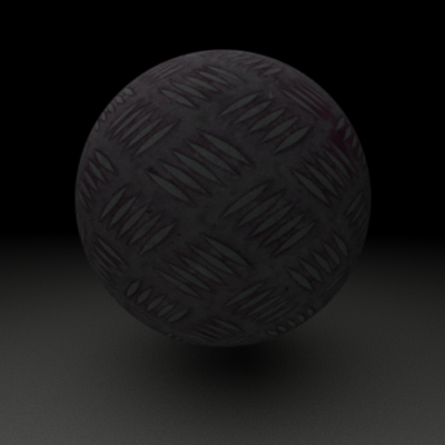
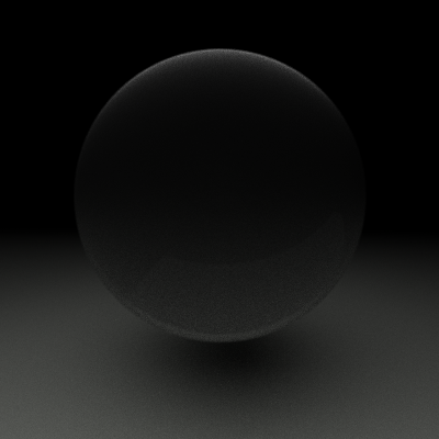
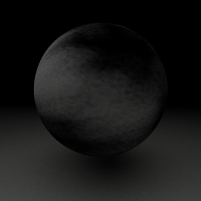
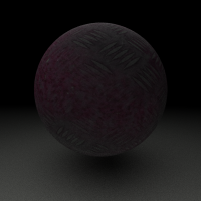
| + | These shade trees scale to as many levels as the effect requires. The final image at the bottom of this post shows an image using several modules. A Heyney-Greenstein module provides a shiny metallic surface. Another is a texture module to provide the metal surface. These modules must be combined in a combo filter separately from the rust so that the rust doesn't appear shiny. This combo filter is fed into a mask filter with the rust as it's other shader. A texture module is fed into the mask filter to use as the mask. | ||
| + | |||
| + | [[File:im_synth_p14_metal.png|frame|center|The sphere with just the metal texture]] | ||
| + | |||
| + | [[File:im_synth_p14_hg.png|frame|center|The sphere using the Heyney-Greenstein module]] | ||
| + | |||
| + | [[File:im_synth_p14_rust.png|frame|center|The sphere with just the rust texture]] | ||
| + | |||
| + | [[File:im_synth_p14_mask.png|frame|center|The sphere using the mask texture]] | ||
| + | |||
| + | [[File:im_synth_p14_combo.png|frame|center|The final sphere using the entire shade tree described above. This gives the overall feel of the metal, while splotching rust on parts in a natural-looking splat]] | ||
Latest revision as of 07:31, 18 January 2015
I took this class with Dr. Pete Shirley in 2006. He was a very animated professor and loved talking about light and how it behaved. At one point I remember him mid sentence running into the kitchen connected to our classroom and coming back with a glass container he held up looking at it from different angles to talk about refraction.
All of the assignments were completed via blog postings. I decided to write my renderer in java for kicks, while most people chose to use C++. Looking back I slightly regret my decision since I had no experience writing "fast" java code and my renders took noticeably longer than my classmates. Still it was one of the funnest college courses I had.
Contents
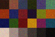
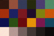
Project 1
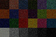
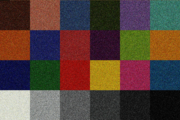
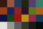
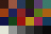
This first project samples various frequencies on the Macbeth color checker. If it passes a basic sampling check, the image color is sampled to the frame buffer. All the samples are acculumated over each time step to get a better average color. All these images were rendered at 720x480 (they seemed like good numbers). They were rendered on a Toshiba Tecra S2.
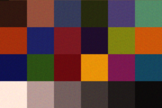
Project 2
This second project is similar to the first. I sampled XYZ estimates using the tristimulus curves and converted the samples on the graphics card to RGB using the Adobe RGB table conversion standard matrix. It took my poor little laptop almost two minutes to render 1024 time steps at 720x480.
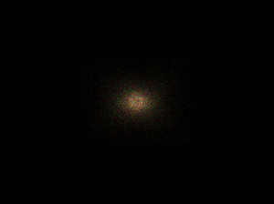
Project 3
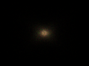
These are samples from a simulated sensor. The grid is on the xy-plane and a sphere emitting light from it's surface at random vectors hits the sensor grid and accumulates XYZ factors, which are converted to RGB on the graphics card and displayed to the screen. Below are images of this program taken at different number of photon emissions.
Project 4 and 5
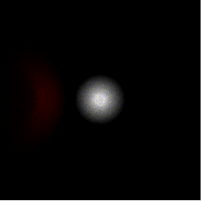
In the previous project, a single sphere-shaped light emitter was placed onto the sensor grid. In the example, the light source has been moved back and a pinhole has been added between the sensor grid and all other objects in the scene. This pinhole only allows vectors of photons pass through it if it they travel inside the pinhole to reach the grid. Other photons are thrown out. This pinhole-camera scheme provides a much better detailed picture than the previous implementation as it simulates a perspective frustrum just like the eye or a real camera. A red diffuse sphere bounces light from the light source to the pinhole also.
Included in this project was an importance sampling implementation. This fired photons at the diffuse sphere and directly at the pinhole. The amount of photons fired to each object was a ratio of their solid angle and the total number of photons previously fired in all directions. Because only photons sent to the pinhole and the object were fired, the scene was rendered using much fewer photons. Although more overhead was required to calculate the importance sampling, it greatly reduced the calculation time for every photon collision (having much fewer photons in the scene).
Both of these projects were added to the previous code base at the same time. Importance sampling was required to provide an more interactive debugging of the pinhole code. Final images look better than the previous project, and took much less time to synthesize.
Project 6 and 15
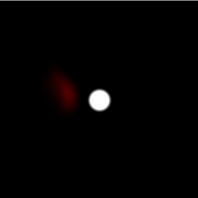
In Project 4 & 5, the imager was modified to handle importance sampling and a pinhole camera. The importance sampling provided much faster rendering times by sending photons only at known objects in the scene, and weighting them based on their angle. The photons were generated at the sensor grid and sent through the scene until they hit a light source (or bounced too much). This seemed to provide a good sampling of the scene, but required a major rewrite of the code.
This new version of the software adds a lens to the scene as well as motion blur. To handle motion blur, the red diffuse sphere was moved from (0, 1, 3) to (1, 2, 4) over the course of the rendering. This created an easy but interesting blur effect as if the object was exposed over many sensor units while the apperture was open.
The lense was a simple biconvex lense attached to the pinhole. Upon contact with the lense, the vector was skewed based on it's angle of incidence and the refractive index of the lense (1.4 for this lense). As the photon left this lense, it would be skewed again. Snell's law was used to calculate the angles of refraction for each photon.
Project 7 and 8
In Project 7, we were to use our renderer to model the Cornell box. This box was compared against a physical model to compare accuracy in the rendering software. This scene's walls and light are modeled using the geometry data and color data from the Cornell box at http://www.graphics.cornell.edu/online/box/data.html.
In addition to the light source and the walls, Project 8 added fresnel effects to the renderer. Instead of the two blocks found in the original Cornell box, two diffuse spheres have been placed in the far corners of the room. A large transparent sphere is placed in the center of the room, which shows the light refracting through it.
The scene's light seems rather blurry because it was moved down slightly to not create artifacts with the ceiling, which is one giant polygon.
Project 9
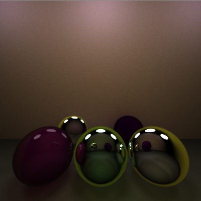
In Project 9, we were to add the Beere-Lambert Law to our renderer. The Beere-Lambert Law models the amount of light absorbed while traveling through a medium. Because different wavelengths are absorbed based on the distance they must travel through the medium, different colors can be absorbed causing different wavelengths to be more pronounced. Certain types of glass often absorb high and low wavelengths leaving a greenish tint at certain angles. Usually this effect can be seen when the light is going through the greatest distance of the glass. To compute the absorbtion at certain frequencies, euler's number e was taken to the exponent of the distance times a large negative constant (which changes based on the scene metrics).
In the picture below, five spheres are modeled. The back left sphere is a reflective sphere, while the back right is a diffuse sphere. Theses spheres are only to provide background to the scene. The spheres in front are used for comparison. The left sphere is a diffuse/reflective sphere with a purplish hue. The middle sphere is a translucent sphere that implements the Beere-Lambert Law based on the distance of the medium. This gives the sphere the slightly greenish tint. The sphere on the right is also a translucent sphere, but does not implement the Beere-Lambert Law. This was to show the difference in hues generated by this principle.
Project 10
In Project 10, we were to implement participating media. Participating media involves computing physical bounces of light in media such as fog, dust, smoke, etc. where the light bounces around inside the volume instead of just diffusing, reflecting, or refracting.
To implement this, I used the standard marching technique through an axis-aligned bounding box. A ray was sampled multiple times across its vector using small steps. When these steps were inside the bounding volume, they probabilisitcally hit some of the media.
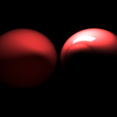
Project 11
In Project 11, subsurface scattering is added to the renderer. This implies that light hitting the surface of the material enters and bounces around inside the medium before exiting. Many materials such as grapes, skin and marble exhibit this quality. Subsurface scattering in this implementation used ray marching, where the ray enters the medium and bounces around until exiting. Because the ray actually bounced around inside the object instead of just off the surface, the rendering was far more computationally expensive than rendering this scene without SSC.
Project 12
In Project 12, the Heyney-Greenstein Phase Function was implemented in the renderer. The Heyney-Greenstein Phase Function (HGPF) is an imperical formula to simulate diffuse and specular reflection for a variety of materials using only two parameters. This function uses these these two parameters stored in each object and takes the incidence angle as input. This provides a much greater flexibility for different materials than using the simpler Lambertian reflection.
Finding little data as to proper values, I rendered an image using a wide range of values. From the image generated, it appears a high g-value seems important to produce a good image. This component supposedly relates directly to the angle where most of the light is leaving. It seems natural that a g-value closer to 1 will produce better pictures where light bounces off at a 90-degree angle, while a 0 value gives very splotchy results. The w-value used in the function scales the function and seems to have less of an effect after tone mapping is appled.
Project 14
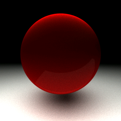
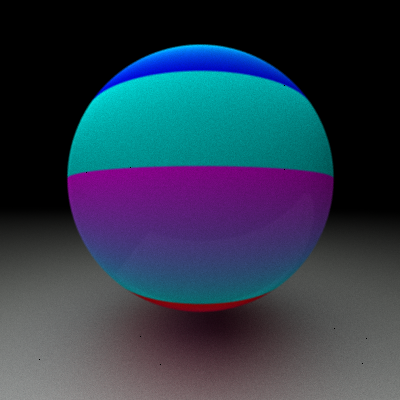
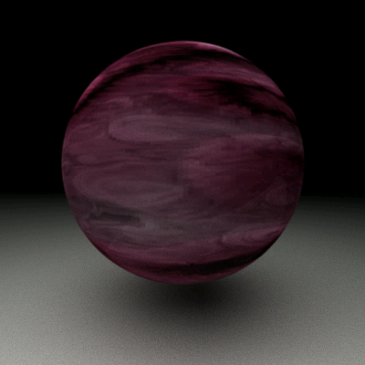
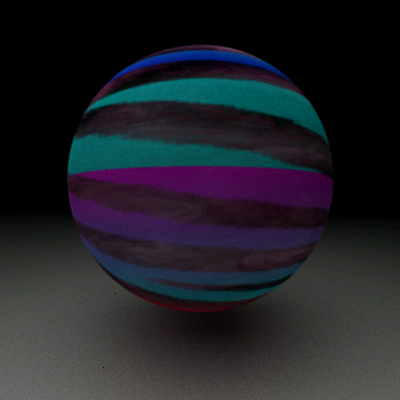
In Project 14, for my "cool effect" I implemented shade trees. Shade trees provide a procedural, modular workflow for determining a color at a given point based on various parameters similar to the ones needed in the Heyney-Greenstein Phase Function.
These shade trees allow simple modules to be built and combined in chains or branches. Some common shade trees provide basic shading effects like Phong shading, Lambertian shading, anisotropic shading, ramp shading, etc. Other modules allow combinations and filters to provide more complex images using these simple modules.
Below are a few different spheres using some shading modules...
These shade trees scale to as many levels as the effect requires. The final image at the bottom of this post shows an image using several modules. A Heyney-Greenstein module provides a shiny metallic surface. Another is a texture module to provide the metal surface. These modules must be combined in a combo filter separately from the rust so that the rust doesn't appear shiny. This combo filter is fed into a mask filter with the rust as it's other shader. A texture module is fed into the mask filter to use as the mask.
